Damage cell quality control
Compiled: 2025-10-19
Source:vignettes/detailed-detection-vignette.Rmd
detailed-detection-vignette.RmdTutorial overview
The goal of DamageDetective is to simplify the process
of making informed and reproducible damaged cell filtering decisions.
This tutorial provides an outline of the steps needed to achieve
this:
Data preparation
Parameter selection
Damaged cell detection
Ensure the following packages are installed and made available in your R environment to follow along:
-
DamageDetective,ggplot2,Seurat,SeuratData,scRNAseq,SingleCellExperiment, andpatchwork.
Workflow overview
The DamageDetective workflow is made up of two stages,
first, creating artificial profiles of damage using the cells of an
input data set, and second, comparing the input cells to the artificial
profiles.
This approach is inspired by DoubletFinder—a
high-performing tool for filtering doublets, another prominent scRNA-seq
artifact. Here, artificial profiles of doublets are created through the
random combination of existing cells. All cells are processed before
being compared in a principal component analysis (PCA) from which
proximity measures are taken and used to determine the proportion of a
true cell’s neighbours that are of artificial origin (proportion of
artificial nearest neighbours, or pANN). Cells that show the highest
pANN, i.e., have the highest proximity to artificial profiles, are
ultimately labelled as doublets in accordance to anticipated doublet
formation rate.
In DamageDetective, a score is similarly calculated for
each cell based on PCA comparisons where scores closer to one indicate a
greater proximity to artificially profiles and a higher likelihood of
damage. This score is used to filter cells, either automatically using
the default threshold or manually according to a user-defined
threshold.
How these scores are calculated and what exactly they describe will be explored briefly before heading into the demonstrations.
Creating artificial damage
The loss of plasma membrane integrity is a characteristic of cellular damage that has long since been exploited to assess cell viability. Compromised membranes allow cellular content, including RNA, to escape, leading to shifts in quality control metrics such as a reduction in library size and complexity.
An additional and fundamental consequence of membrane integrity loss
is a shift in library composition. This occurs because not all RNA
within a cell is equally vulnerable to loss. RNA enclosed by additional
membranes, such as within mitochondria or nuclear speckles, is more
protected than RNA freely present in the cytoplasm. As a result, viable
cells have a higher proportion of cytoplasmic RNA, whereas damaged
cells—where RNA has escaped—appear to have an elevated proportion of
protected RNA. This forms the basis for simulating damage in
DamageDetective.
Artificial damage profiles are generated by simulating the loss of cytoplasmic RNA to reflect varying levels of cellular damage. Each artificial cell is assigned a target damage level between 0 and 1, drawn from a normal distribution centered between 0.65 and 1. This range is based on the assumption that losing at least 65 % of cytoplasmic RNA represents a substantial level of damage warranting exclusion from downstream analysis. To simulate this, transcripts are sampled from each cell without replacement, according to gene abundance within the cell, until the desired proportion of RNA loss is achieved.
Simulations are grouped by cluster from the input data to generate cell type–specific profiles of damage. The goal is to create a pool of artificially damaged cells that reflects all cell types present in a heterogeneous sample. Depending on the target damage level, these artificial cells retain some of the original gene expression signatures of their cell type while exhibiting features typical of damage—such as reduced complexity, smaller library sizes, and increased mitochondrial RNA—resulting from the simulated loss of cytoplasmic RNA. This provides a realistic basis for comparison and, ultimately, a means of estimating true damage.
Estimating true damage by comparison to artificial damage
DamageDetective estimates the damage level of true cells
by measuring their similarity to artificially damaged cells. Like
DoubletFinder, this measurement is rooted in PCA. However,
instead of using full gene expression values, it uses cell quality
control (QC) metrics, including library size, complexity, and
mitochondrial RNA proportion—a biologically informative and
computationally efficient alternative.
Using Euclidean distances between the PCA embeddings of cells, a set
of
nearest neighbours is identified for each cell via the HNSW
(Hierarchical Navigable Small World) algorithm. This is optimized for
high-dimensional data and implemented in R using C++ through the
RcppHNSW package.
The proportions of a cell’s nearest neighbours that originate from each artificial profile (pANN) are calculated. In other words, if there are five clusters in a dataset, there will be five sets of artificial profiles and five pANN scores for each cell. After scaling according to the size of each artificial profile, the maximum pANN is retrieved for each cell. This score naturally lies between 0 and 1 and indicates the similarity of true cells to damaged profiles.
The proximity score forms the main output of
DamageDetective and can be thought of as answering the
question: on a scale of 0 to 1, how likely is it that this cell has lost
a considerable amount of cytoplasmic RNA? Or, equivalently, how likely
is it that this cell is damaged and should be filtered?
Data preparation
DamageDetective operates with single cell data in the
form of a compressed, column-oriented sparse matrix
(dgCMatrix) in R. This format efficiently
handles the sparse nature of single cell data by indexing only non-zero
elements within each column, i.e., only the rows containing actual
expression values. We will begin by showing how three common single cell
data storage types can be converted to this form to act as the starting
point for damage detection.
These include,
- Alignment output files
-
Seuratobject -
SingleCellExperiment(sce) object
Convert data to sparse matrix format
1. Alignment output
Alignment output comes in the form of three files,
-
features.tsv, containing the gene names
-
barcodes.tsv, containing the cell identifiers
-
matrix.mtx, containing the input values (gene expression values).
These can be compiled using ReadMtx offered by
Seurat which simplifies the count matrix compilation
process into one function. This includes the processes of decompressing
zipped files, mapping feature names to HGNC gene symbols, and converting
the matrix to sparse format. The ReadMtx() output can be
used directly as input for DamageDetective.
We will use publicly available alignment data from the 10X Genomics website for demonstration, specifically the ‘1k PBMCs from a healthy donor (v3)’ dataset, which can be downloaded here following the link named “Feature / cell matrix (filtered)”. This should begin the download of a 9.6 MB directory containing ‘filtered_feature_bc_matrix’ sub-directory housing the alignment files.
# Set the file paths relative to location on your device
matrix_file <- "~/Projects/filtered_feature_bc_matrix/matrix.mtx.gz"
barcodes_file <- "~/Projects/filtered_feature_bc_matrix/barcodes.tsv.gz"
features_file <- "~/Projects/filtered_feature_bc_matrix/features.tsv.gz"

# Construct the sparse matrix
alignment_counts <- Seurat::ReadMtx(
  mtx = matrix_file,
  cells = barcodes_file,
  features = features_file
)
Note: Please adjust the location,
~/Projects, according to where the files are saved on your device.
2. Seurat object
Seurat is one of the most popular packages for single
cell analysis in R. Along with an extensive suite of
functions, it offers its own S4 class of data storage for housing the
count matrix, aptly named the Seurat object. By default,
the count matrix is already in compressed column-oriented sparse form in
the Seurat object and can be used as input for
DamageDetective after it is extracted from the assay
slot.
You can use the SeuratData package to retrieve a
publicly available Seurat object to test this. This object
stores the data from peripheral blood mononuclear cells (PBMCs)
sequenced using the 10X Genomics platform.
3. sce object
Bioconductor offers its own suite of packages for single
cell analysis in R with their own single cell data storage type known as
the SingleCellExperiment (sce) object. Here,
the count matrix is stored as a delayed matrix. This format enables
memory-efficient operations by delaying computations until
explicitly requested, rather than storing all values in memory upfront.
However, DamageDetective computations require repeated
access to the matrix and delays at each request greatly accumulate to
slow down this process. We therefore convert the delayed matrix to a
sparse matrix via a dense matrix intermediate.
You can use the scRNAseq package to retrieve a publicly
available sce object to test this. This object stores PBMC
data of multiple samples from a study investigating influenza and yellow
fever vaccine responsiveness. We will focus on the “234_d0” sample
coming from an individual with a high vaccine responsiveness.
if (!require("BiocManager", quietly = TRUE))
    install.packages("BiocManager")
BiocManager::install("scRNAseq")
library(scRNAseq)

# Retrieve multisample dataset
pbmc_sce <- scRNAseq::fetchDataset("kotliarov-pbmc-2020", "2024-04-18")

# Extract sample of interest
metadata <- SummarizedExperiment::colData(pbmc_sce)
sample_sce <- subset(metadata, sample == "234_d0")
sample_sce <- rownames(sample_sce)

# Subset and convert to sparse format
pbmc_counts <- SummarizedExperiment::assay(pbmc_sce, "counts")
sample_counts  <- pbmc_counts[, sample_sce]
sample_counts <- as.matrix(sample_counts)
sample_counts <- as(sample_counts, "dgCMatrix")
Note: Like many single cell analysis packages, DamageDetective can only operate with one single cell dataset at a time. Hence why we work with only the “234_d0” sample above.
Parameter selection
Once the count matrix is in the correct format, the
detect_damage function of DamageDetective can
be run immediately. However, detect_damage accepts
additional parameters. These parameters can be divided into two
categories, those that alter the computation and result in a different
output, computational parameters, and those that adjust
how the user receives the output but cannot change the output itself,
aesthetic parameters. Both will be explored
briefly.
Computational parameters
Dataset-defined computational parameters
Of the parameters that affect the output of the detection algorithm, some have only one possible input based on the data being investigated. In many cases, these require no alteration from the defaults. These include,
| Parameter | Default | Description |
|---|---|---|
organism |
"Hsap" |
Specifies the organism the data was derived from. Supports
"Hsap" (human) and "Mmus" (mouse). |
annotated_celltypes |
FALSE |
Indicates whether cell types are already annotated. If
TRUE, ensures simulations are distributed evenly across
known cell types. |
To use a non-default organism, specify the strings used to identify mitochondrial and ribosomal genes, and optionally, a set of nuclear-enriched genes.
For example, the format for human data is:
User-defined computational parameters
The remaining computational parameters have a wider range of input
possibilities. While the user is free to adjust these as they see fit,
we recommend using the defaults provided as they resulted in consistent
and intended performance during package development. This being said,
the ribosome_penalty parameter must be adjusted according
to the input data and is explored in more detail below.
| Parameter | Default | Description |
|---|---|---|
seed |
User-defined | Ensures reproducibility of the algorithm. While the seed affects random sampling, its impact is minimal unless using cells with unusually high expression and low sparsity. |
kN |
One third of the dataset size | Number of nearest neighbours considered when calculating the proportion of nearby damaged cells. Higher values increase chance of false detection due to unrelated artificial neighbours. |
target_damage |
c(0.65, 1) |
Range of cytoplasmic RNA loss used to simulate damage. Higher values simulate more severely damaged cells, forming the basis of the comparison with true cells. |
pca_columns |
c("log.features", "log.counts", "mt.prop", "rb.prop") |
Variables used for principal component analysis during damage detection. Includes traditional and novel quality control metrics and transformations. |
filter_threshold |
0.5 |
Score threshold (0 to 1) used to determine which cells are removed. Lower values enforce stricter filtering, while higher values are more permissive. |
ribosome_penalty |
0.5 | Adjusts the likelihood of ribosomal RNA loss during simulation, correcting for observed discrepancies where ribosomal RNA is retained more than expected. |
Computing the ideal ribosome_penalty
ribosome_penalty is a value between 0 and 1 that is
multiplied by the probability scores of ribosomal RNA loss, reducing the
scores and making it less likely for the ribosomal transcripts to be
sampled for loss.
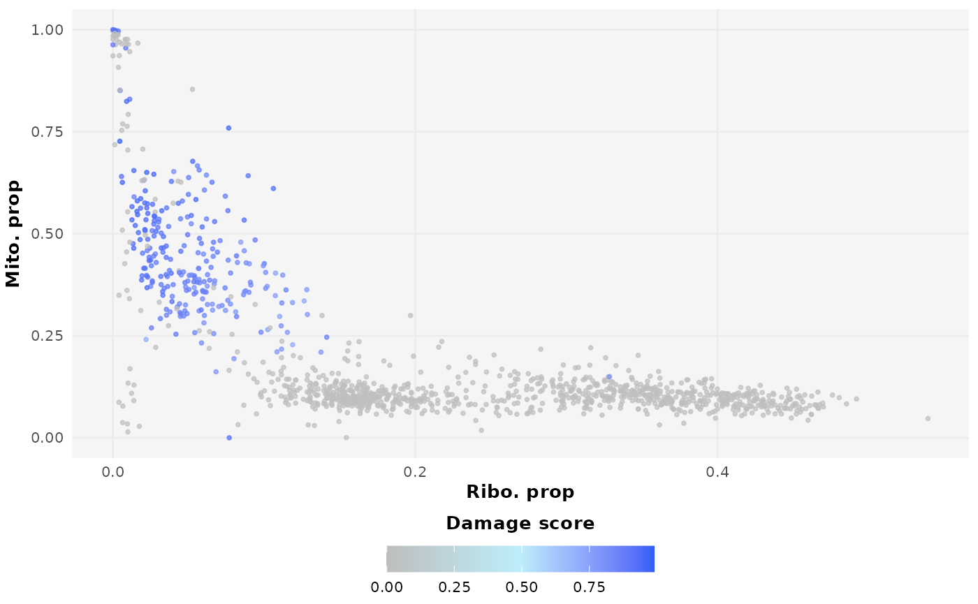
The impact of changing ribosome_penalty can be explored
using the plots generated from simulate_counts below. The
idea here is to see how well the artificial cells generated with a
selected penalty describe the true cells. In other words, how well the
coloured dots superimpose the grey dots. You will see that as you
increase the penalty, i.e. go from values closer to 1 to values closer
to 0, the coloured dots shift from an extreme position on the left-hand
side of the plot to a more central position. At what point along this
range true cells exist is dataset-dependent but generally lies closer to
0. Where,
-
count_matrixis the data in a sparse matrix format as prepared above, -
ribosome_penaltyis a numeric between 0 and 1, and -
damage_proportionis a number between 0 and 1 specifying the amount of artificial cells to create relative to the input data (setting this to a lower value makes the computation faster).
no_penalty <- DamageDetective::simulate_counts(
  count_matrix = alignment_counts,
  ribosome_penalty = 1,
  damage_proportion = 0.25,
  target_damage = c(0.6, 1),
  plot_ribosomal_penalty = TRUE,
  seed = 7
)

no_penalty_plot <- no_penalty$plot + ggtitle("No penalty") +
  theme(plot.title = element_text(face = "bold", hjust = 0.5))

medium_penalty <- DamageDetective::simulate_counts(
  count_matrix = alignment_counts,
  ribosome_penalty = 0.2,
  damage_proportion = 0.25,
  target_damage = c(0.6, 1),
  plot_ribosomal_penalty = TRUE,
  seed = 7
)

med_penalty_plot <- medium_penalty$plot +
  ggtitle("Average penalty (0.2)") +
  theme(plot.title = element_text(face = "bold", hjust = 0.5))

high_penalty <- DamageDetective::simulate_counts(
  count_matrix = alignment_counts,
  ribosome_penalty = 0.01,
  damage_proportion = 0.25,
  target_damage = c(0.6, 1),
  plot_ribosomal_penalty = TRUE,
  seed = 7
)

high_penalty_plot <- high_penalty$plot +
  ggtitle("Heavy penalty (0.01)") +
  theme(plot.title = element_text(face = "bold", hjust = 0.5))

no_penalty_plot | med_penalty_plot | high_penalty_plot ribosome_penalty is a multiplicative reduction factor meaning a value of 1 is the same as introducing no penalty while values increasingly closer to zero introduce increasingly greater reductions.
From the above plots you can see how selecting an unideal
ribosome_penalty can generate damaged profiles that do not
describe the data well and, as a result, generate estimations of damage
that do not describe the data well.
Selecting a ribosome_penalty that simulates RNA loss in
a way that is relevant to the input data can be done through trial and
error, similar to the plotting exercise above, or in an automated
fashion using the select_penalty function,
penalty <- DamageDetective::select_penalty(
  count_matrix = alignment_counts,
  max_penalty_trials = 5,
  seed = 7,
  verbose = TRUE
)
#> Testing penalty of 0.1...
#> Testing penalty of 0.15...
#> Testing penalty of 0.2...
#> Testing penalty of 0.25...
#> Stopping early: dTNN is no longer improving.
penalty
#> [1] 0.15
As seen above, the select_penalty function generates
artificial cells using different ribosome_penalty estimates
and evaluates the similarity of the resulting artificial cells to true
cells.
Here, ‘similarity’ refers to the shortest distance from each
artificial cell to a true cell in PC space. The mean shortest distances
are taken for each level of damage simulated. The penalty that generates
the smallest mean distance across damage levels is selected as the ideal
ribosome_penalty. In other words, a penalty that generates
artificial cells that are the most similar to true cells over a wide
range of damage levels is ideal. This can be viewed in greater detail by
setting the return_output parameter to
"full".
selected_penalty <- DamageDetective::select_penalty(
  count_matrix = alignment_counts,
  max_penalty_trials = 5,
  seed = 7,
  return_output = "full",
  verbose = TRUE
)

# View full results
selected_penalty$penalty_results

# View selected penalty (lowest global mean)
selected_penalty$selected_penalty
#> Penalty Global_mean Mean_3 Mean_4 Mean_5 Mean_6
#> 1 0.10 0.07205541 0.04395754 0.04783755 0.06005843 0.13636814
#> 2 0.15 0.04990311 0.03003056 0.04784675 0.05462734 0.06710781
#> 3 0.20 0.05339491 0.03922892 0.04730901 0.05555464 0.07148706
#> 4 0.25 0.05346742 0.03445152 0.05333923 0.06202791 0.06405101
#> [1] 0.15Though not strictly necessary, the select_penalty
function can be adjusted to give a user more control over the testing
process. This includes,
-
penalty_rangesetting a specific range ofribosome_penaltyestimates -
max_penalty_trialsset a maximum number of attempts allowed -
penalty_stepsetting the difference between each estimate -
return_outputreturns a table showing the mean distances for each estimate giving a better idea of how the estimates differ.
select_penalty inherits additional parameters from the
simulate_counts function that control other aspects of the
damage simulation.
Aesthetic parameters
The remaining parameters control how the user receives the final output.
| Parameter | Default | Description |
|---|---|---|
filter_counts |
TRUE |
If TRUE, returns only the filtered count matrix based
on damage classifications using filter_threshold. If
FALSE, returns a data frame of damage scores per barcode
for manual filtering or inspection. |
palette |
User-defined | Allows customization of the color palette used in damage score plots. Must be a vector of three colors indicating low to high damage severity. |
penalty_plot <- DamageDetective::simulate_counts(
  count_matrix = alignment_counts,
  ribosome_penalty = selected_penalty$selected_penalty,
  damage_proportion = 0.2,
  target_damage = c(0.4, 1),
  plot_ribosomal_penalty = TRUE,
  palette = c("grey", "#BCEEFB", "#325EF7"),
  seed = 7
)
Damaged cell detection
Once the data is in sparse matrix form and an appropriate
ribosome_penalty is selected, the
detect_damage function can be run. Below, we have selected
the default filter_counts=FALSE option to view the output
directly.
# Run detection
detection_output <- DamageDetective::detect_damage(
  count_matrix = alignment_counts,
  ribosome_penalty = selected_penalty$selected_penalty,
  seed = 7
)
#> Clustering cells...
#> Checking clusters...
#> Simulating damage...
#> Computing pANN...
#> Suggested pANN threshold : 0.39039039039039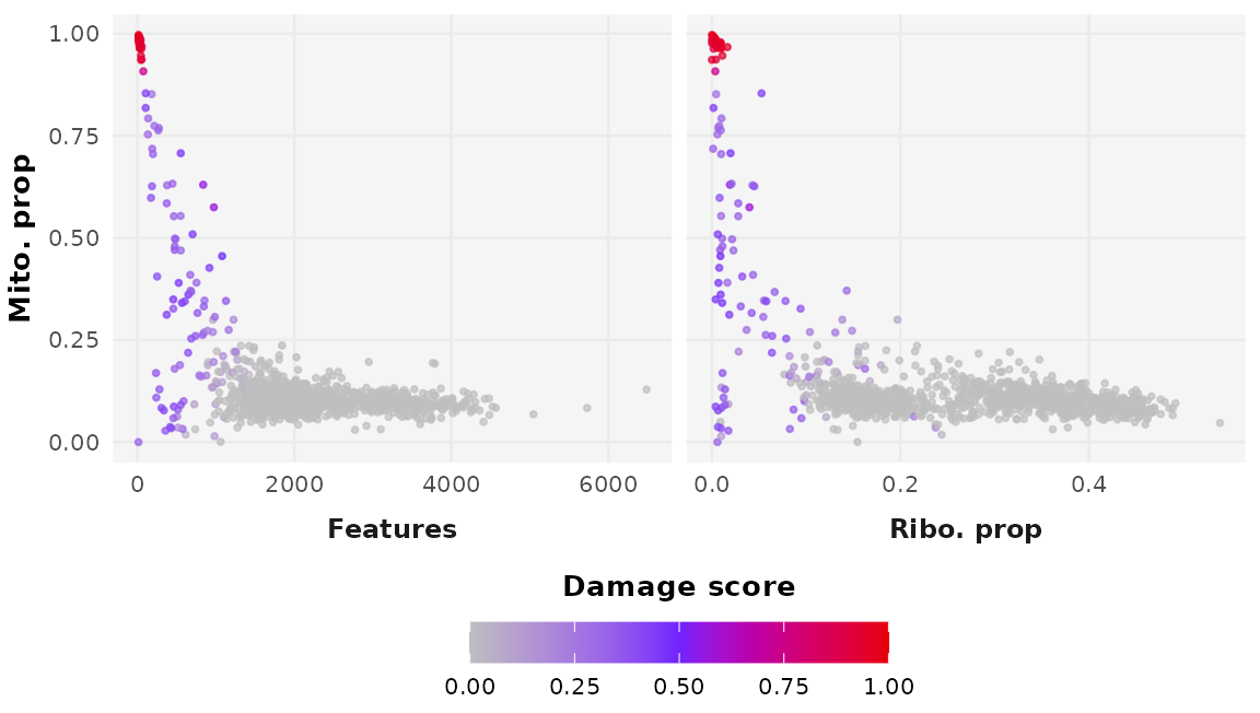
#> Completed.

# View output
head(detection_output$output)
#>                                 Cells DamageDetective pANN
#> AAACCCAAGGAGAGTA-1 AAACCCAAGGAGAGTA-1               0 cell
#> AAACGCTTCAGCCCAG-1 AAACGCTTCAGCCCAG-1               0 cell
#> AAAGAACAGACGACTG-1 AAAGAACAGACGACTG-1               0 cell
#> AAAGAACCAATGGCAG-1 AAAGAACCAATGGCAG-1               0 cell
#> AAAGAACGTCTGCAAT-1 AAAGAACGTCTGCAAT-1               0 cell
#> AAAGGATAGTAGACAT-1 AAAGGATAGTAGACAT-1               0 cell
From here, the matrix can be filtered according to a threshold damage value before continuing with the remainder of pre-processing steps required for a single cell analysis.
undamaged_cells <- subset(detection_output$output, DamageDetective <= 0.5)
filtered_matrix <- alignment_counts[, row.names(undamaged_cells)]
dim(alignment_counts)
#> [1] 13287  1222
dim(filtered_matrix)
#> [1] 13287  1102
This could be done automatically if
filter_counts=TRUE.
# Run detection
filtered_output <- DamageDetective::detect_damage(
  count_matrix = alignment_counts,
  ribosome_penalty = selected_penalty$selected_penalty,
  filter_counts = TRUE,
  generate_plot = FALSE,
  seed = 7
)

dim(filtered_output)
#> [1] 13287 1102Session Information
#> R version 4.5.1 (2025-06-13)
#> Platform: x86_64-pc-linux-gnu
#> Running under: Ubuntu 24.04.3 LTS
#>
#> Matrix products: default
#> BLAS:   /usr/lib/x86_64-linux-gnu/openblas-pthread/libblas.so.3
#> LAPACK: /usr/lib/x86_64-linux-gnu/openblas-pthread/libopenblasp-r0.3.26.so;  LAPACK version 3.12.0
#>
#> locale:
#>  [1] LC_CTYPE=C.UTF-8       LC_NUMERIC=C           LC_TIME=C.UTF-8
#>  [4] LC_COLLATE=C.UTF-8     LC_MONETARY=C.UTF-8    LC_MESSAGES=C.UTF-8
#>  [7] LC_PAPER=C.UTF-8       LC_NAME=C              LC_ADDRESS=C
#> [10] LC_TELEPHONE=C         LC_MEASUREMENT=C.UTF-8 LC_IDENTIFICATION=C
#>
#> time zone: UTC
#> tzcode source: system (glibc)
#>
#> attached base packages:
#> [1] stats     graphics  grDevices utils     datasets  methods   base
#>
#> other attached packages:
#> [1] future_1.67.0          patchwork_1.3.2        ggplot2_4.0.0
#> [4] stringr_1.5.2          Seurat_5.3.0           SeuratObject_5.2.0
#> [7] sp_2.2-0               DamageDetective_2.0.15
#>
#> loaded via a namespace (and not attached):
#>   [1] RColorBrewer_1.1-3     jsonlite_2.0.0         magrittr_2.0.4
#>   [4] spatstat.utils_3.2-0   farver_2.1.2           rmarkdown_2.30
#>   [7] fs_1.6.6               ragg_1.5.0             vctrs_0.6.5
#>  [10] ROCR_1.0-11            spatstat.explore_3.5-3 rstatix_0.7.2
#>  [13] htmltools_0.5.8.1      broom_1.0.10           Formula_1.2-5
#>  [16] sass_0.4.10            sctransform_0.4.2      parallelly_1.45.1
#>  [19] KernSmooth_2.23-26     bslib_0.9.0            htmlwidgets_1.6.4
#>  [22] desc_1.4.3             ica_1.0-3              plyr_1.8.9
#>  [25] plotly_4.11.0          zoo_1.8-14             cachem_1.1.0
#>  [28] igraph_2.2.0           mime_0.13              lifecycle_1.0.4
#>  [31] pkgconfig_2.0.3        Matrix_1.7-3           R6_2.6.1
#>  [34] fastmap_1.2.0          fitdistrplus_1.2-4     shiny_1.11.1
#>  [37] digest_0.6.37          tensor_1.5.1           RSpectra_0.16-2
#>  [40] irlba_2.3.5.1          textshaping_1.0.4      ggpubr_0.6.2
#>  [43] labeling_0.4.3         progressr_0.17.0       spatstat.sparse_3.1-0
#>  [46] httr_1.4.7             polyclip_1.10-7        abind_1.4-8
#>  [49] compiler_4.5.1         proxy_0.4-27           withr_3.0.2
#>  [52] S7_0.2.0               backports_1.5.0        carData_3.0-5
#>  [55] fastDummies_1.7.5      ggsignif_0.6.4         MASS_7.3-65
#>  [58] tools_4.5.1            lmtest_0.9-40          httpuv_1.6.16
#>  [61] future.apply_1.20.0    goftest_1.2-3          glue_1.8.0
#>  [64] nlme_3.1-168           promises_1.3.3         grid_4.5.1
#>  [67] Rtsne_0.17             cluster_2.1.8.1        reshape2_1.4.4
#>  [70] generics_0.1.4         gtable_0.3.6           spatstat.data_3.1-8
#>  [73] class_7.3-23           tidyr_1.3.1            data.table_1.17.8
#>  [76] car_3.1-3              spatstat.geom_3.6-0    RcppAnnoy_0.0.22
#>  [79] ggrepel_0.9.6          RANN_2.6.2             pillar_1.11.1
#>  [82] spam_2.11-1            RcppHNSW_0.6.0         later_1.4.4
#>  [85] splines_4.5.1          dplyr_1.1.4            lattice_0.22-7
#>  [88] survival_3.8-3         deldir_2.0-4           tidyselect_1.2.1
#>  [91] miniUI_0.1.2           pbapply_1.7-4          knitr_1.50
#>  [94] gridExtra_2.3          scattermore_1.2        xfun_0.53
#>  [97] matrixStats_1.5.0      stringi_1.8.7          lazyeval_0.2.2
#> [100] yaml_2.3.10            evaluate_1.0.5         codetools_0.2-20
#> [103] tibble_3.3.0           cli_3.6.5              uwot_0.2.3
#> [106] xtable_1.8-4           reticulate_1.43.0      systemfonts_1.3.1
#> [109] jquerylib_0.1.4        Rcpp_1.1.0             globals_0.18.0
#> [112] spatstat.random_3.4-2  png_0.1-8              spatstat.univar_3.1-4
#> [115] parallel_4.5.1         pkgdown_2.1.3          dotCall64_1.2
#> [118] listenv_0.9.1          viridisLite_0.4.2      scales_1.4.0
#> [121] ggridges_0.5.7         e1071_1.7-16           purrr_1.1.0
#> [124] rlang_1.1.6            cowplot_1.2.0
References
- Amezquita R, et al. (2020). “Orchestrating single-cell analysis with Bioconductor.” Nature Methods, 17, 137-145.
- Hao et al. (2023). Seurat V5. Nature Biotechnology.
- McGinnis, C. S., Murrow, L. M., & Gartner, Z. J. (2019). “DoubletFinder: Doublet Detection in Single-Cell RNA Sequencing Data Using Artificial Nearest Neighbors”. Cell Systems, 8(4), 329-337.e4.
- Pedersen T (2024). patchwork: The Composer of Plots. R package version 1.3.0.
- Satija R, et al. (2025). SeuratData: Install and Manage Seurat Datasets. R package version 0.2.2.9002.
- Wickham. ggplot2: Elegant Graphics for Data Analysis. Springer-Verlag New York, 2016.